5.5. Bayesian Model Mixing using Gaussian Processes: Stationary Kernel Tutorial

5.5.1. Author: Alexandra C. Semposki

5.5.1.1. Date: 02 July 2026

Welcome to the tutorial notebook for using the new gp-bmm method in Taweret! Here we will overview what the method does and how to use it on a toy model. We will assume the user has some familiarity with Gaussian processes (GPs); if not, one can check out this Jupyter Book, which contains some introductory material on GPs and preliminary exercises.

This tutorial specifically handles the so-called “stationary” kernel, which uses the Euclidean distance between points in the input space as the main input to the kernel. In the next notebook, we will cover the scenario where distance is not sufficient information and we need to include structure from the input space in our kernel construction.

Below, we set up the toy model that we will be using, the so-called “SAMBA models”, and then construct a stationary, squared-exponential radial basis function (RBF) kernel that will be used to mix the two models we have chosen. We will also cover the inclusion of a hyperprior on the hyperparameters of this kernel, so that we obtain better physically-motivated results, which will be extremely useful for realistic physics applications.

The core of this work was included in Taweret from this paper and this paper, written by A. C. Semposki et al., and the accompanying package, neutron-rich-bmm, originally found here.

from matplotlib.ticker import AutoMinorLocator
from sklearn.gaussian_process.kernels import RBF, ConstantKernel as C

import Taweret.mix.gp_bmm as T_gp
import Taweret.models.samba_models as samba

We use model code defined in the Taweret.models subpackage to define the models we would like to perform model mixing on.

# now we write out the models we need
models = {
    "hi": samba.Highorder(order=4),
    "lo": samba.Loworder(order=3)
}

Once these models have been initialized, we need to evaluate their results before we apply a model mixing strategy.

# predict functions for the plot
g = np.linspace(1e-6, 1.0, 100)
predict = [
    models["lo"].evaluate(g),
    models["hi"].evaluate(g)
]
predict_labels = [rf'$N_s={models["lo"].order}$', rf'$N_l={models["hi"].order}$']

#basic plot to check choices
fig = plt.figure(figsize=(8,6), dpi=100)
ax = plt.axes()
ax.set_xlim(0.0,1.0)
ax.set_ylim(1.2,3.2)
ax.tick_params(axis='x', direction='in')
ax.tick_params(axis='y', direction='in')
ax.locator_params(nbins=8)
ax.xaxis.set_minor_locator(AutoMinorLocator())
ax.yaxis.set_minor_locator(AutoMinorLocator())
ax.set_title('SAMBA Models')
ax.set_xlabel('g')
ax.set_ylabel('F(g)')

#truth
ax.plot(g, samba.TrueModel().evaluate(g)[0].flatten(), 'k', label='True')

#models with uncertainties
for i in range(len(predict)):
    ax.plot(g, predict[i][0].flatten(), color=COLORS[i], linestyle=LINES[0], label=predict_labels[i])
    ax.plot(g, predict[i][0].flatten() - predict[i][1].flatten(), color=COLORS[i], linestyle=LINES[1])
    ax.plot(g, predict[i][0].flatten() + predict[i][1].flatten(), color=COLORS[i], linestyle=LINES[1])

_ = ax.legend()

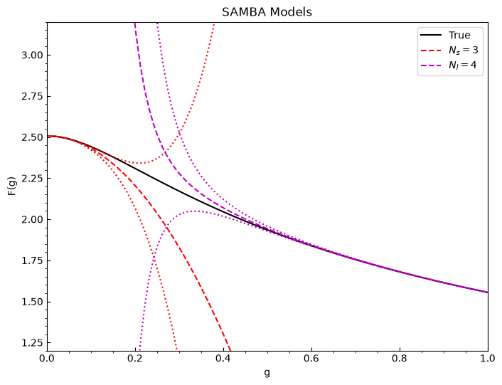
Because the method we wish to use, the GP-BMM strategy, requires that we possess not only means and standard deviations at each data point from the models, but also the covariance matrix of the model at those points, we will construct a toy covariance matrix for both models. In reality, this information should hopefully already be present in the physics model. If it is not, one can do an estimation as below to try to emulate the expected covariance.

def build_cov_from_errors(x, sigma, ell=10.0, nugget=1e-6):
    x = np.asarray(x)
    sigma = np.asarray(sigma)

    dx = x[:, None] - x[None, :]
    rho = np.exp(-0.5 * (dx / ell)**2)

    C = np.outer(sigma, sigma) * rho
    C += nugget * np.eye(len(x))
    return C

# take some training data from these, and make some covariances up for the toy case
x_lo = g[:30:5]
x_hi = np.append(g[40:-1:5], g[-1])

# cut the data as well
data_lo = predict[0][0][:30:5]
sigma_lo = predict[0][1][:30:5]
data_hi = np.append(predict[1][0][40:-1:5], predict[1][0][-1])
sigma_hi = np.append(predict[1][1][40:-1:5], predict[1][1][-1])

# try the covariance function here
cov_lo = build_cov_from_errors(x_lo, sigma_lo, ell=0.1, nugget=1e-6)
cov_hi = build_cov_from_errors(x_hi, sigma_hi, ell=1.0, nugget=1e-6)

#basic plot to check choices
fig = plt.figure(figsize=(8,6), dpi=100)
ax = plt.axes()
ax.set_xlim(0.0,1.0)
ax.set_ylim(1.2,3.2)
ax.tick_params(axis='x', direction='in')
ax.tick_params(axis='y', direction='in')
ax.locator_params(nbins=8)
ax.xaxis.set_minor_locator(AutoMinorLocator())
ax.yaxis.set_minor_locator(AutoMinorLocator())
ax.set_title('SAMBA Models')
ax.set_xlabel('g')
ax.set_ylabel('F(g)')

#truth
ax.plot(g, samba.TrueModel().evaluate(g)[0].flatten(), 'k', label='True')

#models with uncertainties
for i in range(len(predict)):
    ax.plot(g, predict[i][0].flatten(), color=COLORS[i], linestyle=LINES[0], label=predict_labels[i])
    ax.plot(g, predict[i][0].flatten() - predict[i][1].flatten(), color=COLORS[i], linestyle=LINES[1])
    ax.plot(g, predict[i][0].flatten() + predict[i][1].flatten(), color=COLORS[i], linestyle=LINES[1])

# add data and covariances
ax.errorbar(x_lo, data_lo, sigma_lo, marker='.', color=COLORS[0], linestyle=' ')
ax.errorbar(x_hi, data_hi, sigma_hi, marker='.', color=COLORS[1], linestyle=' ')

_ = ax.legend()

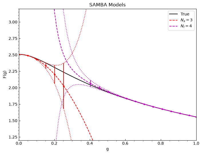
# concatenate the training data
x_train = np.concatenate((x_lo, x_hi)).reshape(-1,1)
y_train = np.concatenate((data_lo,data_hi)).reshape(-1,1)

# covariance matrix
alpha = scipy.linalg.block_diag(cov_lo, cov_hi)

Now we have our training data, so let’s try to construct a valid stationary GP for this problem that is able to capture the underlying truth. We begin by choosing the default priors that the mixing class already contains.

# now we make a kernel to send to the class using typical scikit-learn notation
kernel = C(
    constant_value=1.1,
    constant_value_bounds=[0.25,2.25]) * RBF(length_scale=0.05, length_scale_bounds=[0.02,0.1]
)

With the kernel defined for the GP, we then call the mixing method from the Taweret.mix subpackage; this is called the GPmixing class.

# load the class for mixing with no prior assumptions
bmm = T_gp.GPmixing(g, models=models, alpha=alpha, kernel=kernel,
                    priors=True, prior_params=None, prior_choice='rbfnorm')

unconstrained_prior = bmm.prior_predict()
assert all(unconstrained_prior["mean"] == 0.0)

In the above, we notice that the mean is zero. This is because we haven’t actually conditioned the GP on the training data, so it has no information about the data yet. We’ve simply calculated what the prior might give us across the regime given the kernel we have defined. Hence, it is often better to return the draws from this distribution, since they will show us the spread of the prior better than the prior parameter choices will. We do this below and plot the draws.

# draw from the prior
_, draws = bmm.prior_predict(sample=True, n_samples=10)

#basic plot to check choices
fig = plt.figure(figsize=(8,6), dpi=100)
ax = plt.axes()
ax.set_xlim(0.0,1.0)
ax.tick_params(axis='x', direction='in')
ax.tick_params(axis='y', direction='in')
ax.locator_params(nbins=8)
ax.xaxis.set_minor_locator(AutoMinorLocator())
ax.yaxis.set_minor_locator(AutoMinorLocator())
ax.set_title('Prior draws')
ax.set_xlabel('g')
ax.set_ylabel('F(g)')
_ = ax.plot(g, draws)

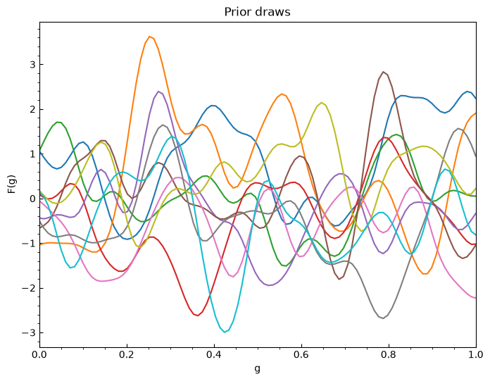
We can also evaluate the prior using the evaluate function, which we can do before any training has happened.

evalprior = bmm.evaluate(x_train)

Then we can train the hyperparameters of the GP kernel, and produce our BMM result. We do this by using the train function in the GPMixing class.

bmm.train(x_train, y_train)

print('Initial kernel:', bmm.gpr.kernel)
print('Trained kernel:', bmm.gpr.kernel_)

Initial kernel: 1.05**2 * RBF(length_scale=0.05)
Trained kernel: 0.914**2 * RBF(length_scale=0.0997)

We can see that the values have indeed changed and the calibration is finished. We note that since we asked for priors to be applied via priors=True in our class definition, we have used the default priors of the Taweret code to obtain this result. The form of the default priors is the truncated normal distribution,

\[ \theta_i | I \sim \mathcal{U}(a_i, b_i) \times \mathcal{N}(\mu_i, \sigma_i), \]

where \(\theta_i\) are the hyperparameters of the GP kernel, and the hard cutoffs \(a_i\) and \(b_i\) can be chosen for physical reasons, e.g., to limit the correlation length of the GP based on physical knowledge of the system, etc. \(\mu_i\) and \(\sigma_i\) are also chosen to provide a starting guess of what the hyperparameters should be.

The values of these optimized hyperparameters are shown below.

# reveal default priors
print(bmm.prior_params)

{'sigma': {'mu': 1.0, 'sig': 0.25}, 'lengthscale': {'mu': 1.0, 'sig': 0.15}}

Now that the training has been completed, let’s look at the predictions from this result. We plot them over the original models for comparison.

# let's predict with this kernel now
predictions = bmm.predict()

# check the keys of the dict
print(predictions.keys())

dict_keys(['x', 'mean', 'std', 'cov'])

# plot these results over the original models and the data
fig = plt.figure(figsize=(8,6), dpi=100)
ax = plt.axes()
ax.set_xlim(0.0,1.0)
ax.set_ylim(1.2,3.2)
ax.tick_params(axis='x', direction='in')
ax.tick_params(axis='y', direction='in')
ax.locator_params(nbins=8)
ax.xaxis.set_minor_locator(AutoMinorLocator())
ax.yaxis.set_minor_locator(AutoMinorLocator())
ax.set_title('SAMBA Models')
ax.set_xlabel('g')
ax.set_ylabel('F(g)')

#truth
ax.plot(g, samba.TrueModel().evaluate(g)[0].flatten(), 'k', label='True')

#models with uncertainties
for i in range(len(predict)):
    ax.plot(g, predict[i][0].flatten(), color=COLORS[i], linestyle=LINES[0], label=predict_labels[i])
    ax.plot(g, predict[i][0].flatten() - predict[i][1].flatten(), color=COLORS[i], linestyle=LINES[1])
    ax.plot(g, predict[i][0].flatten() + predict[i][1].flatten(), color=COLORS[i], linestyle=LINES[1])

# add data and covariances
ax.errorbar(x_lo, data_lo, sigma_lo, marker='.', color=COLORS[0], linestyle=' ')
ax.errorbar(x_hi, data_hi, sigma_hi, marker='.', color=COLORS[1], linestyle=' ')

# GP results
ax.plot(predictions['x'], predictions['mean'], color='mediumpurple', label='GP prediction')
ax.fill_between(predictions['x'], predictions['mean']-predictions['std'],
                predictions['mean']+predictions['std'], color='mediumpurple', alpha=0.2)

_ = ax.legend()

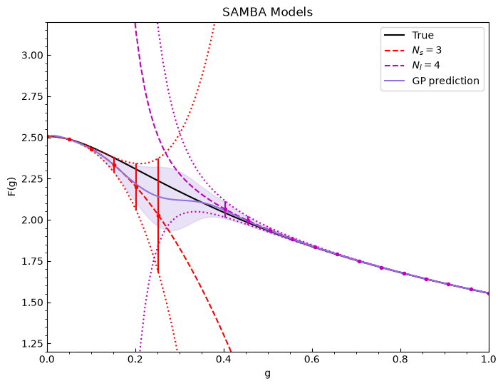
print('Optimized parameters:', bmm.map)

Optimized parameters: [0.83600701 0.09965627]

Now we test using different prior definitions instead of the default parameters; this for now doesn’t mean we choose a different prior form, rather, we change our mean and variance values of the truncated Gaussian that is being used under the hood here. However, different forms can also be specified—priors can be given to Taweret by the user through generating and including a priors.py file in the utils folder.

For now, to simply change the values of the hyperprior forms, e.g., the mean and variance, we need to define the priors we wish to choose here, or we can use the default prior settings incorporated into Taweret.

prior_params = {
    'sigma': {'mu': 1.0, 'sig': 0.25},
    'lengthscale': {'mu': 0.1, 'sig': 0.05}
}

# try running this code with input prior params dicts
bmm2 = T_gp.GPmixing(g, models=models, alpha=alpha, kernel=kernel,
                     priors=True, prior_params=prior_params, prior_choice='rbfnorm')

bmm2.train(x_train, y_train)
predictionspriors = bmm2.predict()

# plot these results over the original models and the data
fig = plt.figure(figsize=(8,6), dpi=100)
ax = plt.axes()
ax.set_xlim(0.0,1.0)
ax.set_ylim(1.2,3.2)
ax.tick_params(axis='x', direction='in')
ax.tick_params(axis='y', direction='in')
ax.locator_params(nbins=8)
ax.xaxis.set_minor_locator(AutoMinorLocator())
ax.yaxis.set_minor_locator(AutoMinorLocator())
ax.set_title('SAMBA Models')
ax.set_xlabel('g')
ax.set_ylabel('F(g)')

#truth
ax.plot(g, samba.TrueModel().evaluate(g)[0].flatten(), 'k', label='True')

#models with uncertainties
for i in range(len(predict)):
    ax.plot(g, predict[i][0].flatten(), color=COLORS[i], linestyle=LINES[0], label=predict_labels[i])
    ax.plot(g, predict[i][0].flatten() - predict[i][1].flatten(), color=COLORS[i], linestyle=LINES[1])
    ax.plot(g, predict[i][0].flatten() + predict[i][1].flatten(), color=COLORS[i], linestyle=LINES[1])

# add data and covariances
ax.errorbar(x_lo, data_lo, sigma_lo, marker='.', color=COLORS[0], linestyle=' ')
ax.errorbar(x_hi, data_hi, sigma_hi, marker='.', color=COLORS[1], linestyle=' ')

# GP results
ax.plot(predictions['x'], predictions['mean'], color='mediumpurple', label='GP prediction w/default priors')
ax.fill_between(predictions['x'], predictions['mean']-predictions['std'],
                predictions['mean']+predictions['std'], color='mediumpurple', alpha=0.2)

ax.plot(predictionspriors['x'], predictionspriors['mean'], color='forestgreen', label='GP prediction w/custom priors')
ax.fill_between(predictionspriors['x'], predictionspriors['mean']-predictionspriors['std'],
                predictionspriors['mean']+predictionspriors['std'], color='forestgreen', alpha=0.2)

_ = ax.legend()

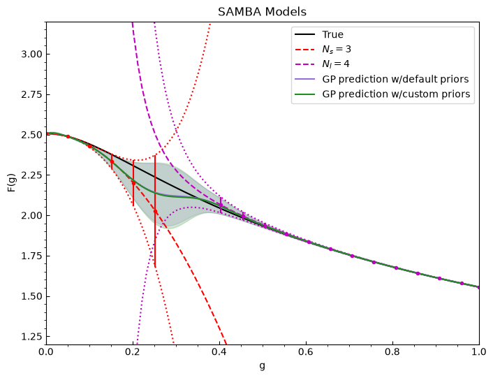
We can see above the slight difference between this model and the one we trained using the default priors. One can continue to play with the possibilities to determine which constraints are most physically meaningful for the problem at hand. For now, we hope this tutorial helped you get used to the capabilities of the GPMixing module in Taweret!