5.6. Bayesian Model Mixing using Gaussian Processes: Nonstationary Kernel Tutorial

5.6.1. Author: Alexandra C. Semposki

5.6.1.1. Date: 02 July 2026

Welcome to the second tutorial for the Gaussian process (GP) model mixing module in Taweret! Here we present an example of using a nonstationary kernel for your GP prior on the function space. This will entail designing a custom kernel in scikit-learn. We include in Taweret the custom kernel we have used to generate the results in this paper; of course, if you wish, you may design your own custom kernel and add it to the file kernels.py that we have included here in the utils folder.

Let’s first load the toy models we will be using.

from matplotlib.ticker import AutoMinorLocator
from sklearn.gaussian_process.kernels import RBF, ConstantKernel as C

import Taweret.mix.gp_bmm as T_gp
import Taweret.utils.kernels as T_kernels
import Taweret.models.samba_models as samba

5.6.2. Setting up the models

# now we write out the models we need
models = {
    "lo": samba.Loworder(order=3),
    "hi": samba.Highorder(order=4)
}

# predict functions for the plot
g = np.linspace(1e-6, 1.0, 100)
predict = [
    models["lo"].evaluate(g),
    models["hi"].evaluate(g)
]
predict_labels = [rf'$N_s={models["lo"].order}$', rf'$N_l={models["hi"].order}$']

# basic plot to check choices
fig = plt.figure(figsize=(8,6), dpi=100)
ax = plt.axes()
ax.set_xlim(0.0,1.0)
ax.set_ylim(1.2,3.2)
ax.tick_params(axis='x', direction='in')
ax.tick_params(axis='y', direction='in')
ax.locator_params(nbins=8)
ax.xaxis.set_minor_locator(AutoMinorLocator())
ax.yaxis.set_minor_locator(AutoMinorLocator())
ax.set_title('SAMBA Models')
ax.set_xlabel('g')
ax.set_ylabel('F(g)')

# truth
ax.plot(g, samba.TrueModel().evaluate(g)[0].flatten(), 'k', label='True')

# models with uncertainties
for i in range(len(predict)):
    ax.plot(g, predict[i][0].flatten(), color=COLORS[i], linestyle=LINES[0], label=predict_labels[i])
    ax.plot(g, predict[i][0].flatten() - predict[i][1].flatten(), color=COLORS[i], linestyle=LINES[1])
    ax.plot(g, predict[i][0].flatten() + predict[i][1].flatten(), color=COLORS[i], linestyle=LINES[1])

_ = ax.legend()

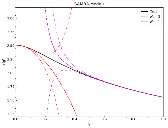
We first need to build the covariance matrix again since we will need to train a GP with knowledge of input-space correlations.

def build_cov_from_errors(x, sigma, ell=10.0, nugget=1e-6):
    x = np.asarray(x)
    sigma = np.asarray(sigma)

    dx = x[:, None] - x[None, :]
    rho = np.exp(-0.5 * (dx / ell)**2)

    C = np.outer(sigma, sigma) * rho
    C += nugget * np.eye(len(x))
    return C

# take some training data from these, and make some covariances up for the toy case
x_lo = g[:30:3]
x_hi = np.append(g[40:-1:5], g[-1])

# cut the data as well
data_lo = predict[0][0][:30:3]
sigma_lo = predict[0][1][:30:3]
data_hi = np.append(predict[1][0][40:-1:5], predict[1][0][-1])
sigma_hi = np.append(predict[1][1][40:-1:5], predict[1][1][-1])

# try the covariance function here
cov_lo = build_cov_from_errors(x_lo, sigma_lo, ell=0.1, nugget=1e-6)
cov_hi = build_cov_from_errors(x_hi, sigma_hi, ell=1.0, nugget=1e-6)

# build full alpha covariance matrix for the GPmixing step
xtot = np.concatenate((x_lo, x_hi))
datatot = np.concatenate((data_lo, data_hi))
alpha = scipy.linalg.block_diag(cov_lo, cov_hi)

#basic plot to check choices
fig = plt.figure(figsize=(8,6), dpi=100)
ax = plt.axes()
ax.set_xlim(0.0,1.0)
ax.set_ylim(1.2,3.2)
ax.tick_params(axis='x', direction='in')
ax.tick_params(axis='y', direction='in')
ax.locator_params(nbins=8)
ax.xaxis.set_minor_locator(AutoMinorLocator())
ax.yaxis.set_minor_locator(AutoMinorLocator())
ax.set_title('SAMBA Models')
ax.set_xlabel('g')
ax.set_ylabel('F(g)')

#truth
ax.plot(g, samba.TrueModel().evaluate(g)[0].flatten(), 'k', label='True')

#models with uncertainties
for i in range(len(predict)):
    ax.plot(g, predict[i][0].flatten(), color=COLORS[i], linestyle=LINES[0], label=predict_labels[i])
    ax.plot(g, predict[i][0].flatten() - predict[i][1].flatten(), color=COLORS[i], linestyle=LINES[1])
    ax.plot(g, predict[i][0].flatten() + predict[i][1].flatten(), color=COLORS[i], linestyle=LINES[1])

# add data and covariances
ax.errorbar(x_lo, data_lo, sigma_lo, marker='.', color=COLORS[0], linestyle=' ')
ax.errorbar(x_hi, data_hi, sigma_hi, marker='.', color=COLORS[1], linestyle=' ')

_ = ax.legend()

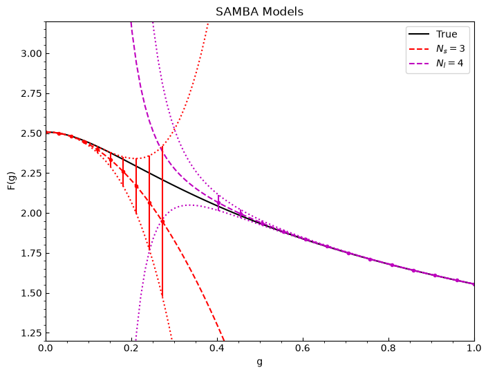
5.6.3. GP frozen kernels for the two models

Now we will design what we will call a nonstationary kernel, which means it will depend on the input space (here, on our location in \(g\)). To do this, we first will define frozen GP kernels that will emulate our models. We do this here because it allows us to quickly design a kernel that has the necessary positive-definite characteristic the GP relies on. We do this below by defining our frozen kernels and plotting their results on top of our models. These frozen kernels are RBF kernels with a ConstantKernel to absorb the marginal variance.

# write the frozen GP kernels
k1_ls = 0.15
k1_c2 = 500.0
k1 = C(constant_value=k1_c2,
       constant_value_bounds='fixed') * RBF(length_scale=k1_ls, length_scale_bounds='fixed')

# directly feed GPRwrapper the kernel and alpha here
gp1 = T_gp.GPRwrapper(
    kernel=k1,
    alpha = cov_lo,
)

gp1.fit(x_lo.reshape(-1,1), data_lo.reshape(-1,1))

print(gp1.kernel_)

gp1_predict, gp1_cov_predict = gp1.predict(g.reshape(-1,1), return_cov=True)
gp1_std_predict = np.sqrt(np.diag(gp1_cov_predict))

# plot the result quickly to test
fig = plt.figure(figsize=(8,6), dpi=100)
ax = plt.axes()
ax.set_xlim(0.0,0.5)
ax.set_ylim(1.2,3.2)
ax.tick_params(axis='x', direction='in')
ax.tick_params(axis='y', direction='in')
ax.locator_params(nbins=8)
ax.xaxis.set_minor_locator(AutoMinorLocator())
ax.yaxis.set_minor_locator(AutoMinorLocator())
ax.set_title('SAMBA Models')
ax.set_xlabel('g')
ax.set_ylabel('F(g)')

#truth
ax.plot(g, samba.TrueModel().evaluate(g)[0].flatten(), 'k', label='True')

#model with uncertainties
ax.plot(g, predict[0][0].flatten(), color=COLORS[0], linestyle=LINES[0], label=predict_labels[0])
ax.plot(g, predict[0][0].flatten() - predict[0][1].flatten(), color=COLORS[0], linestyle=LINES[1])
ax.plot(g, predict[0][0].flatten() + predict[0][1].flatten(), color=COLORS[0], linestyle=LINES[1])

# add data and covariances
ax.errorbar(x_lo, data_lo, sigma_lo, marker='.', color=COLORS[0], linestyle=' ')

# GP prediction
ax.plot(g, gp1_predict, color=COLORS[0], label='GP prediction')
ax.fill_between(g,
                gp1_predict - gp1_std_predict,
                gp1_predict + gp1_std_predict,
                alpha=0.3, color=COLORS[0])

_= ax.legend()

22.4**2 * RBF(length_scale=0.15)

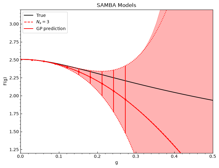
# write the frozen GP kernels
k2_ls = 0.15
k2_c2 = 5.0
k2 = C(constant_value=k2_c2,
       constant_value_bounds='fixed') * RBF(length_scale=k2_ls, length_scale_bounds='fixed')

gp2 = T_gp.GPRwrapper(
    kernel=k2,
    alpha = cov_hi,
)

gp2.fit(x_hi.reshape(-1,1), data_hi.reshape(-1,1))

print(gp2.kernel_)

gp2_predict, gp2_cov_predict = gp2.predict(g.reshape(-1,1), return_cov=True)
gp2_std_predict = np.sqrt(np.diag(gp2_cov_predict))

# plot the result quickly to test
fig = plt.figure(figsize=(8,6), dpi=100)
ax = plt.axes()
ax.set_xlim(0.3, 1.0)
ax.set_ylim(1.5, 2.6)
ax.tick_params(axis='x', direction='in')
ax.tick_params(axis='y', direction='in')
ax.locator_params(nbins=8)
ax.xaxis.set_minor_locator(AutoMinorLocator())
ax.yaxis.set_minor_locator(AutoMinorLocator())
ax.set_title('SAMBA Models')
ax.set_xlabel('g')
ax.set_ylabel('F(g)')

#truth
ax.plot(g, samba.TrueModel().evaluate(g)[0].flatten(), 'k', label='True')

#model with uncertainties
ax.plot(g, predict[1][0].flatten(), color=COLORS[1], linestyle=LINES[0], label=predict_labels[1])
ax.plot(g, predict[1][0].flatten() - predict[1][1].flatten(), color=COLORS[1], linestyle=LINES[1])
ax.plot(g, predict[1][0].flatten() + predict[1][1].flatten(), color=COLORS[1], linestyle=LINES[1])

# add data and covariances
ax.errorbar(x_hi, data_hi, sigma_hi, marker='.', color=COLORS[1], linestyle=' ')

# GP prediction
ax.plot(g, gp2_predict, color=COLORS[1], label='GP prediction')
ax.fill_between(g,
                gp2_predict - gp2_std_predict,
                gp2_predict + gp2_std_predict,
                alpha=0.3, color=COLORS[1])

_ = ax.legend()

2.24**2 * RBF(length_scale=0.15)

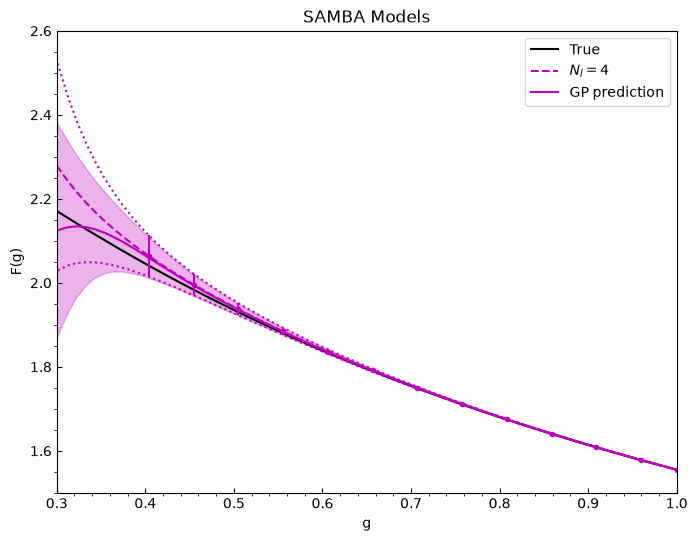
We do not care that this does not match outside of our data region, since we do not trust that region in terms of the original model. Here we are only concerned with matching the behaviour of the data we take from the model, so that we may construct a reasonable changepoint kernel.

5.6.4. Sigmoid mixing function with a changepoint kernel

For our changepoint kernel, we use the form

\[ \kappa(x,x'; x_0, w, \ell_1, \ell_2, \bar{c}^2_1, \bar{c}^2_2) = [1 - \alpha(x; x_0, w)]\kappa_1(x,x';\ell_1,\bar{c}^2_1)[1 - \alpha(x'; x_0, w)] + \alpha(x; x_0, w)\kappa_2(x,x'; \ell_2, \bar{c}^2_2)\alpha(x'; x_0, w), \]

where \(\alpha(x; x_0, w)\) is the sigmoid mixing function

\[ \alpha(x; x_0, w) = \frac{1}{(1 + \exp(-(x-x_0)/w)}. \]

In the following, we use our information to estimate the hyperparameters of the mixing function, the changepoint itself, \(x_0\), and the width over which the kernel transforms, \(w\).

# set up the kernel for the changepoint construction
kernelCP = T_kernels.SigmoidChangepoint(
    ls1=k1_ls, ls2=k2_ls, cbar1=k1_c2, cbar2=k2_c2,
    changepoint=0.3, changepoint_bounds=[0.2, 0.6],
    width=0.2, width_bounds=[0.1, 0.3]
)

# set up prior dict for the different hyperparameters
prior_dict = {
    'w': 'truncnorm',
    'cp': 'truncnorm'
}

# set up the model mixing step
gpmix = T_gp.GPmixing(
    x=g, models=models, alpha=alpha, kernel=kernelCP,
    priors=True, prior_params=None, prior_choice='changepoint', prior_type=prior_dict,
    switch='sigmoid', nopt=5000)

In the above, we have taken prior_params=None, which means we will be using the default hyperpriors set in the code for the changepoint kernel case, since we set prior_choice='changepoint'. A user can of course enter their own priors for the GP to use! The current hyperprior form being used is a truncated normal distribution,

\[ x_0 | I \sim \mathcal{U}(a, b) \times \mathcal{N}(\mu, \sigma), \]

and the same form for the width \(w\). Here, \(a\) and \(b\) can be implemented as hard cutoffs based on physical restrictions from the problem; in our case, we simply would pick something reasonable for the model range we are in so that we do not let the changepoint or width drift too far into the model spaces themselves. \(\mu\) and \(\sigma\) allow us to also control the general range of where we would expect the changepoint or width MAP value to be. This can also be based on physical restrictions; in the toy model, for example, one would expect the changepoint to be around the value \(g=0.3\), since this is where both models are failing.

# fit and predict using the changepoint kernel
gpmix.train(xtot.reshape(-1,1), datatot.reshape(-1,1))
print(gpmix.gpr.kernel_)

gpmix_pred = gpmix.predict()

SigmoidChangepoint(changepoint=0.23, width=0.115)

# plot the resulting predictions
fig = plt.figure(figsize=(8,6), dpi=100)
ax = plt.axes()
ax.set_xlim(0.0,1.0)
ax.set_ylim(1.2,3.2)
ax.tick_params(axis='x', direction='in')
ax.tick_params(axis='y', direction='in')
ax.locator_params(nbins=8)
ax.xaxis.set_minor_locator(AutoMinorLocator())
ax.yaxis.set_minor_locator(AutoMinorLocator())
ax.set_title('SAMBA Models')
ax.set_xlabel('g')
ax.set_ylabel('F(g)')

#truth
ax.plot(g, samba.TrueModel().evaluate(g)[0].flatten(), 'k', label='True')

#models with uncertainties
for i in range(len(predict)):
    ax.plot(g, predict[i][0].flatten(), color=COLORS[i], linestyle=LINES[0], label=predict_labels[i])
    ax.plot(g, predict[i][0].flatten() - predict[i][1].flatten(), color=COLORS[i], linestyle=LINES[1])
    ax.plot(g, predict[i][0].flatten() + predict[i][1].flatten(), color=COLORS[i], linestyle=LINES[1])

# add data and covariances
ax.errorbar(x_lo, data_lo, sigma_lo, marker='.', color=COLORS[0], linestyle=' ')
ax.errorbar(x_hi, data_hi, sigma_hi, marker='.', color=COLORS[1], linestyle=' ')

# add GP predictions with changepoint kernel
ax.plot(gpmix_pred['x'], gpmix_pred['mean'], color=COLORS[2], label='GP prediction w/CP kernel')
ax.fill_between(gpmix_pred['x'],
                gpmix_pred['mean'] - gpmix_pred['std'],
                gpmix_pred['mean'] + gpmix_pred['std'],
                alpha=0.3, color=COLORS[2])

_ = ax.legend()

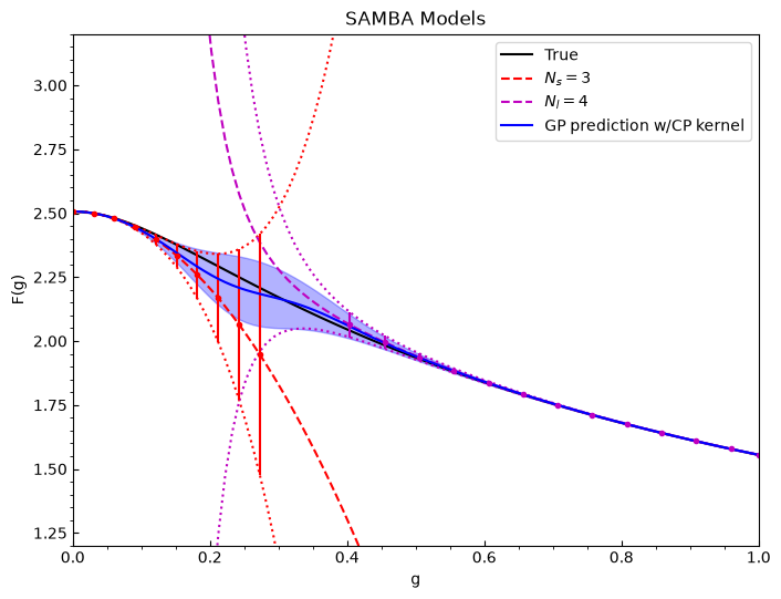
This result correctly captures the uncertainties at the low and high ends of the input space, which we trust from our original models , and produces a result in the intermediate region that smoothly joins the two models together through the changepoint kernel.