2.2. Linear Bivariate BMM with SAMBA toy models : cdf mixing#
The best way to learn Taweret is to use it. You can run, modify and experiment with this notebook on GitHub Codespaces.
This notebook shows how to use the Bayesian model mixing package Taweret for a toy problem.
Author : Dan Liyanage
Date : 11/10/2022
More about SAMBA toy models can be found in Uncertainties here, there, and everywhere: interpolating between small- and large-g expansions using Bayesian Model Mixing
import sys
import os

# You will have to change the following imports depending on where you have
# the packages installed

# ! pip install Taweret    # if using Colab, uncomment to install

cwd = os.getcwd()

# Get the first part of this path and append to the sys.path
tw_path = cwd.split("Taweret/")[0] + "Taweret"
samba_path = tw_path + "/subpackages/SAMBA"
sys.path.append(tw_path)
sys.path.append(samba_path)

# For plotting
import matplotlib.pyplot as plt

! pip install seaborn    # comment if installed
! pip install ptemcee    # comment if installed

import seaborn as sns
sns.set_context('poster')
# To define priors. (uncoment if not using default priors)
# ! pip install bilby   # uncomment this line if bilby is not already installed
import bilby

# For other operations
import numpy as np
Requirement already satisfied: seaborn in /home/runner/work/Taweret/Taweret/.tox/book/lib/python3.13/site-packages (0.13.2)
Requirement already satisfied: numpy!=1.24.0,>=1.20 in /home/runner/work/Taweret/Taweret/.tox/book/lib/python3.13/site-packages (from seaborn) (2.4.6)
Requirement already satisfied: pandas>=1.2 in /home/runner/work/Taweret/Taweret/.tox/book/lib/python3.13/site-packages (from seaborn) (3.0.3)
Requirement already satisfied: matplotlib!=3.6.1,>=3.4 in /home/runner/work/Taweret/Taweret/.tox/book/lib/python3.13/site-packages (from seaborn) (3.11.0)
Requirement already satisfied: contourpy>=1.0.1 in /home/runner/work/Taweret/Taweret/.tox/book/lib/python3.13/site-packages (from matplotlib!=3.6.1,>=3.4->seaborn) (1.3.3)
Requirement already satisfied: cycler>=0.10 in /home/runner/work/Taweret/Taweret/.tox/book/lib/python3.13/site-packages (from matplotlib!=3.6.1,>=3.4->seaborn) (0.12.1)
Requirement already satisfied: fonttools>=4.22.0 in /home/runner/work/Taweret/Taweret/.tox/book/lib/python3.13/site-packages (from matplotlib!=3.6.1,>=3.4->seaborn) (4.63.0)
Requirement already satisfied: kiwisolver>=1.3.1 in /home/runner/work/Taweret/Taweret/.tox/book/lib/python3.13/site-packages (from matplotlib!=3.6.1,>=3.4->seaborn) (1.5.0)
Requirement already satisfied: packaging>=20.0 in /home/runner/work/Taweret/Taweret/.tox/book/lib/python3.13/site-packages (from matplotlib!=3.6.1,>=3.4->seaborn) (26.2)
Requirement already satisfied: pillow>=9 in /home/runner/work/Taweret/Taweret/.tox/book/lib/python3.13/site-packages (from matplotlib!=3.6.1,>=3.4->seaborn) (12.2.0)
Requirement already satisfied: pyparsing>=3 in /home/runner/work/Taweret/Taweret/.tox/book/lib/python3.13/site-packages (from matplotlib!=3.6.1,>=3.4->seaborn) (3.3.2)
Requirement already satisfied: python-dateutil>=2.7 in /home/runner/work/Taweret/Taweret/.tox/book/lib/python3.13/site-packages (from matplotlib!=3.6.1,>=3.4->seaborn) (2.9.0.post0)
Requirement already satisfied: six>=1.5 in /home/runner/work/Taweret/Taweret/.tox/book/lib/python3.13/site-packages (from python-dateutil>=2.7->matplotlib!=3.6.1,>=3.4->seaborn) (1.17.0)
Requirement already satisfied: ptemcee in /home/runner/work/Taweret/Taweret/.tox/book/lib/python3.13/site-packages (1.0.0)
Requirement already satisfied: numpy in /home/runner/work/Taweret/Taweret/.tox/book/lib/python3.13/site-packages (from ptemcee) (2.4.6)
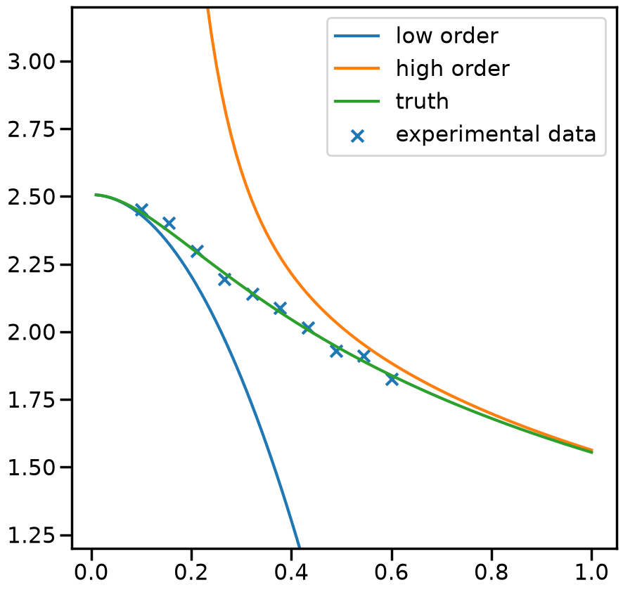
2.2.1. 1. Get toy models and the pseudo-experimental data#
# Toy models from SAMBA
from Taweret.models import samba_models as toy_models

m1 = toy_models.Loworder(2, 'uninformative')
m2 = toy_models.Highorder(2, 'uninformative')
truth = toy_models.TrueModel()
exp = toy_models.Data()
g = np.linspace(0.1, 0.6, 10)
plot_g = np.linspace(0.01,1,100)
m1_prediction = m1.evaluate(plot_g)
m2_prediction = m2.evaluate(plot_g)
true_output = truth.evaluate(plot_g)
exp_data= exp.evaluate(g,error = 0.01)
fig, ax_f = plt.subplots(figsize=(10,10))
ax_f.plot(plot_g, m1_prediction[0].flatten(), label='low order')
ax_f.plot(plot_g, m2_prediction[0].flatten(), label='high order')
ax_f.plot(plot_g, true_output[0], label='truth')
ax_f.scatter(g,exp_data[0], marker='x', label='experimental data')
ax_f.set_ylim(1.2,3.2)
ax_f.legend()
<matplotlib.legend.Legend at 0x7f402138cad0>
2.2.2. 2. Choose a Mixing method#
# Mixing method
from Taweret.mix.bivariate_linear import BivariateLinear as BL

models= {'low_order':m1,'high_order':m2}
mix_model = BL(models_dic=models, method='cdf')
#uncoment to change the prior from the default
priors = bilby.core.prior.PriorDict()
priors['cdf_0'] = bilby.core.prior.Uniform(-20,20, name="cdf_0")
priors['cdf_1'] = bilby.core.prior.Uniform(-20,20, name="cdf_1")
mix_model.set_prior(priors)
{'cdf_0': Uniform(minimum=-20, maximum=20, name='cdf_0', latex_label='cdf_0', unit=None, boundary=None),
 'cdf_1': Uniform(minimum=-20, maximum=20, name='cdf_1', latex_label='cdf_1', unit=None, boundary=None)}
2.2.3. 3. Train to find posterior#
mix_model.prior
{'cdf_0': Uniform(minimum=-20, maximum=20, name='cdf_0', latex_label='cdf_0', unit=None, boundary=None),
 'cdf_1': Uniform(minimum=-20, maximum=20, name='cdf_1', latex_label='cdf_1', unit=None, boundary=None)}
y_exp = np.array(exp_data[0]).reshape(1,-1)
y_err = np.array(exp_data[1]).reshape(1,-1)
# The parameters are set to minimum values for computational ease.
# You should increase the ntemps, nwalkers and nsamples and see
# if your results are changing. If so keep increasing them
# until convergence of results.

kwargs_for_sampler = {'sampler': 'ptemcee',
                    'ntemps': 5,
                    'nwalkers': 50,
                    'Tmax': 100,
                    'burn_in_fixed_discard': 50,
                    'nsamples': 2000,
                    'threads': 6,
                    'verbose':False}

result = mix_model.train(x_exp=g, y_exp=y_exp, y_err=y_err, outdir = 'outdir/samba_bivariate',
label='cdf_mix', kwargs_for_sampler=kwargs_for_sampler)
/home/runner/work/Taweret/Taweret/.tox/book/lib/python3.13/site-packages/bilby/core/likelihood.py:127: FutureWarning: Setting non-trivial parameters for <class 'Taweret.sampler.likelihood_wrappers.likelihood_wrapper_for_bilby'>. This is deprecated behaviour  and will be removed in Bilby version 3. See https://bilby-dev.github.io/bilby/parameters for more details.
  warnings.warn(msg, FutureWarning)
21:43 bilby INFO    : Running for label 'cdf_mix', output will be saved to 'outdir/samba_bivariate'
/home/runner/work/Taweret/Taweret/.tox/book/lib/python3.13/site-packages/bilby/core/sampler/ptemcee.py:134: FutureWarning: The ptemcee sampler interface in bilby is deprecated and will be removed in Bilby version 3. Please use the `ptemcee-bilby`sampler plugin instead: https://github.com/bilby-dev/ptemcee-bilby.
  warnings.warn(msg, FutureWarning)
21:43 bilby INFO    : Analysis priors:
21:43 bilby INFO : cdf_0=Uniform(minimum=-20, maximum=20, name='cdf_0', latex_label='cdf_0', unit=None, boundary=None)
21:43 bilby INFO : cdf_1=Uniform(minimum=-20, maximum=20, name='cdf_1', latex_label='cdf_1', unit=None, boundary=None)
21:43 bilby INFO : Analysis likelihood class: <class 'Taweret.sampler.likelihood_wrappers.likelihood_wrapper_for_bilby'>
21:43 bilby INFO : Analysis likelihood noise evidence: nan
21:43 bilby INFO : Single likelihood evaluation took 3.119e-04 s
21:43 bilby INFO : Using sampler Ptemcee with kwargs {'ntemps': 5, 'nwalkers': 50, 'Tmax': 100, 'betas': None, 'a': 2.0, 'adaptation_lag': 10000, 'adaptation_time': 100, 'random': None, 'adapt': False, 'swap_ratios': False}
21:43 bilby INFO : Global meta data was removed from the result object for compatibility. Use the `BILBY_INCLUDE_GLOBAL_METADATA` environment variable to include it. This behaviour will be removed in a future release. For more details see: https://bilby-dev.github.io/bilby/faq.html#global-meta-data
21:43 bilby INFO : Using convergence inputs: ConvergenceInputs(autocorr_c=5, autocorr_tol=50, autocorr_tau=1, gradient_tau=0.1, gradient_mean_log_posterior=0.1, Q_tol=1.02, safety=1, burn_in_nact=50, burn_in_fixed_discard=50, mean_logl_frac=0.01, thin_by_nact=0.5, nsamples=2000, ignore_keys_for_tau=None, min_tau=1, niterations_per_check=5)
21:43 bilby INFO : Generating pos0 samples
21:43 bilby INFO : Starting to sample
21:44 bilby INFO : Finished sampling
21:44 bilby INFO : Writing checkpoint and diagnostics
21:44 bilby INFO : Finished writing checkpoint
21:44 bilby INFO : Sampling time: 0:01:24.143206
21:44 bilby WARNING : Result.save_to_file called with extension=True. This will default to json, and ignore the extension from the filename. This behaviour is deprecated and will be removed.
21:44 bilby WARNING : Result.save_to_file called with extension=True. This will default to json, and ignore the extension from the filename. This behaviour is deprecated and will be removed.
21:44 bilby INFO    : Summary of results:
nsamples: 2050
ln_noise_evidence:    nan
ln_evidence: -0.149 +/-  2.135
ln_bayes_factor:    nan +/-  2.135
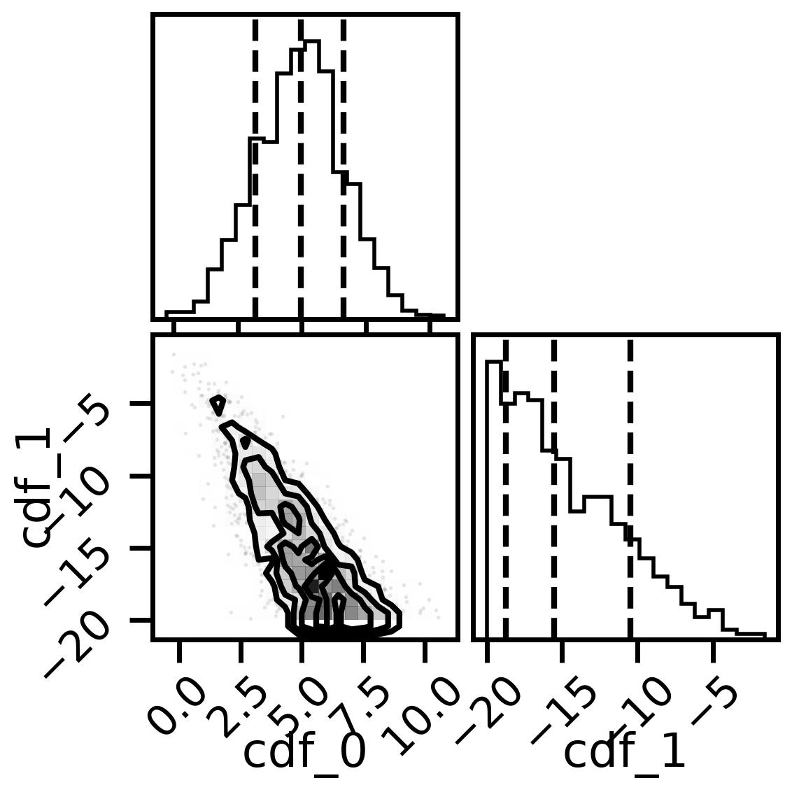
# Posterior of the mixing parameters.
result.plot_corner()

#corner plots
import corner
fig, axs = plt.subplots(2,2, figsize=(6,6), dpi=200)
corner.corner(mix_model.posterior,labels=['cdf_0','cdf_1'],quantiles=[0.16, 0.5, 0.84],fig=fig)
plt.show()
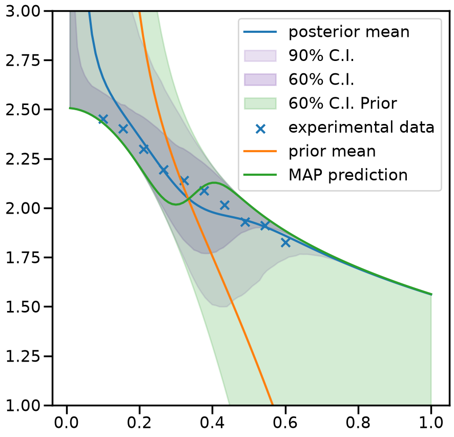
2.2.4. 4. Predictions#
_,mean_prior,CI_prior, _ = mix_model.prior_predict(plot_g, CI=[5,20,80,95])
_,mean,CI, _ = mix_model.predict(plot_g, CI=[5,20,80,95])
per5, per20, per80, per95 = CI
prior5, prior20, prior80, prior95 = CI_prior
# Map value prediction for the step mixing function parameter
map_prediction = mix_model.evaluate(mix_model.map, plot_g)
%matplotlib inline
sns.set_context('poster')
fig, ax = plt.subplots(figsize=(10,10))
ax.plot(plot_g, mean.flatten(), label='posterior mean')
ax.fill_between(plot_g,per5.flatten(),per95.flatten(),color=sns.color_palette()[4], alpha=0.2, label='90% C.I.')
ax.fill_between(plot_g,per20.flatten(),per80.flatten(), color=sns.color_palette()[4], alpha=0.3, label='60% C.I.')
ax.fill_between(plot_g,prior20.flatten(),prior80.flatten(),color=sns.color_palette()[2], alpha=0.2, label='60% C.I. Prior')
ax.scatter(g,exp_data[0], marker='x', label='experimental data')
ax.plot(plot_g, mean_prior.flatten(), label='prior mean')
ax.plot(plot_g, map_prediction.flatten(), label='MAP prediction')
ax.set_ybound(1,3)
ax.legend()
<matplotlib.legend.Legend at 0x7f401c6696d0>