Linear Bivariate BMM with SAMBA toy models : cdf mixing

The best way to learn Taweret is to use it. You can run, modify and experiment with this notebook on GitHub Codespaces.

This notebook shows how to use the Bayesian model mixing package Taweret for a toy problem.

Author : Dan Liyanage

Date : 11/10/2022

More about SAMBA toy models can be found in Uncertainties here, there, and everywhere: interpolating between small- and large-g expansions using Bayesian Model Mixing

import sys
import os

# You will have to change the following imports depending on where you have
# the packages installed

cwd = os.getcwd()

# Get the first part of this path and append to the sys.path
tw_path = cwd.split("Taweret/")[0] + "Taweret"
samba_path = tw_path + "/subpackages/SAMBA"
sys.path.append(tw_path)
sys.path.append(samba_path)

# For plotting
import matplotlib.pyplot as plt
import seaborn as sns
sns.set_context('poster')
# To define priors. (uncoment if not using default priors)
# ! pip install bilby   # uncomment this line if bilby is not already installed
import bilby

# For other operations
import numpy as np

1. Get toy models and the pseudo-experimental data

# Toy models from SAMBA
from Taweret.models import samba_models as toy_models

m1 = toy_models.Loworder(2, 'uninformative')
m2 = toy_models.Highorder(2, 'uninformative')
truth = toy_models.TrueModel()
exp = toy_models.Data()

g = np.linspace(0.1, 0.6, 10)
plot_g = np.linspace(0.01,1,100)
m1_prediction = m1.evaluate(plot_g)
m2_prediction = m2.evaluate(plot_g)
true_output = truth.evaluate(plot_g)
exp_data= exp.evaluate(g,error = 0.01)

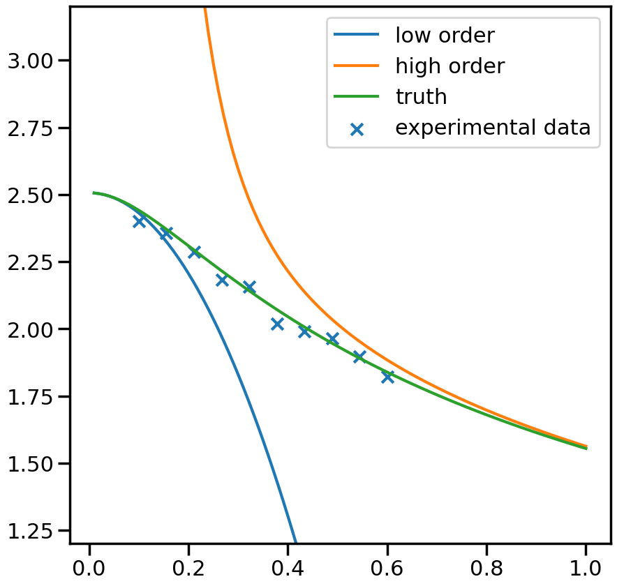
fig, ax_f = plt.subplots(figsize=(10,10))
ax_f.plot(plot_g, m1_prediction[0].flatten(), label='low order')
ax_f.plot(plot_g, m2_prediction[0].flatten(), label='high order')
ax_f.plot(plot_g, true_output[0], label='truth')
ax_f.scatter(g,exp_data[0], marker='x', label='experimental data')
ax_f.set_ylim(1.2,3.2)
ax_f.legend()

<matplotlib.legend.Legend at 0x7fd184a865d0>

2. Choose a Mixing method

# Mixing method
from Taweret.mix.bivariate_linear import BivariateLinear as BL

models= {'low_order':m1,'high_order':m2}
mix_model = BL(models_dic=models, method='cdf')

cdf mixing function has 2                   free parameter(s)
Warning : Default prior is set to {'cdf_0': Uniform(minimum=0, maximum=1, name='cdf_0', latex_label='cdf_0', unit=None, boundary=None), 'cdf_1': Uniform(minimum=0, maximum=1, name='cdf_1', latex_label='cdf_1', unit=None, boundary=None)}
To change the prior use `set_prior` method

#uncoment to change the prior from the default
priors = bilby.core.prior.PriorDict()
priors['cdf_0'] = bilby.core.prior.Uniform(-20,20, name="cdf_0")
priors['cdf_1'] = bilby.core.prior.Uniform(-20,20, name="cdf_1")
mix_model.set_prior(priors)

{'cdf_0': Uniform(minimum=-20, maximum=20, name='cdf_0', latex_label='cdf_0', unit=None, boundary=None),
 'cdf_1': Uniform(minimum=-20, maximum=20, name='cdf_1', latex_label='cdf_1', unit=None, boundary=None)}

3. Train to find posterior

mix_model.prior

{'cdf_0': Uniform(minimum=-20, maximum=20, name='cdf_0', latex_label='cdf_0', unit=None, boundary=None),
 'cdf_1': Uniform(minimum=-20, maximum=20, name='cdf_1', latex_label='cdf_1', unit=None, boundary=None)}

y_exp = np.array(exp_data[0]).reshape(1,-1)
y_err = np.array(exp_data[1]).reshape(1,-1)
# The parameters are set to minimum values for computational ease.
# You should increase the ntemps, nwalkers and nsamples and see
# if your results are changing. If so keep increasing them
# until convergence of results.

kwargs_for_sampler = {'sampler': 'ptemcee',
                    'ntemps': 5,
                    'nwalkers': 50,
                    'Tmax': 100,
                    'burn_in_fixed_discard': 50,
                    'nsamples': 2000,
                    'threads': 6,
                    'printdt': 60}

result = mix_model.train(x_exp=g, y_exp=y_exp, y_err=y_err, outdir = 'outdir/samba_bivariate',
label='cdf_mix', kwargs_for_sampler=kwargs_for_sampler)

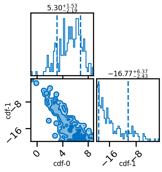
# Posterior of the mixing parameters.
result.plot_corner()

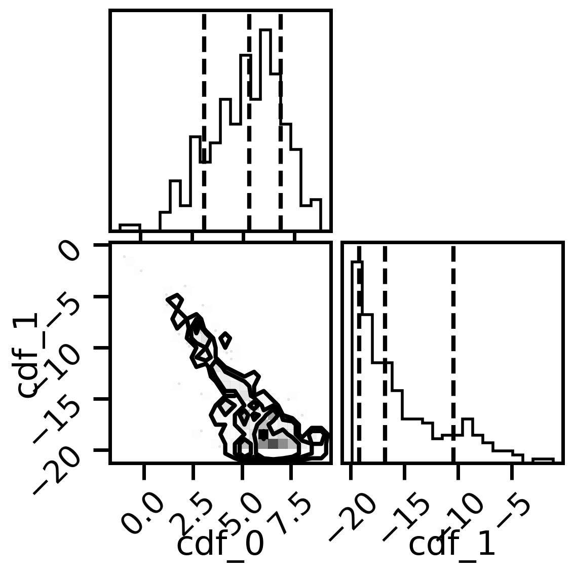
#corner plots
import corner
fig, axs = plt.subplots(2,2, figsize=(6,6), dpi=200)
corner.corner(mix_model.posterior,labels=['cdf_0','cdf_1'],quantiles=[0.16, 0.5, 0.84],fig=fig)
plt.show()

4. Predictions

_,mean_prior,CI_prior, _ = mix_model.prior_predict(plot_g, CI=[5,20,80,95])
_,mean,CI, _ = mix_model.predict(plot_g, CI=[5,20,80,95])

(10000, 2)
using provided samples instead of posterior

per5, per20, per80, per95 = CI
prior5, prior20, prior80, prior95 = CI_prior

# Map value prediction for the step mixing function parameter
map_prediction = mix_model.evaluate(mix_model.map, plot_g)

%matplotlib inline
sns.set_context('poster')
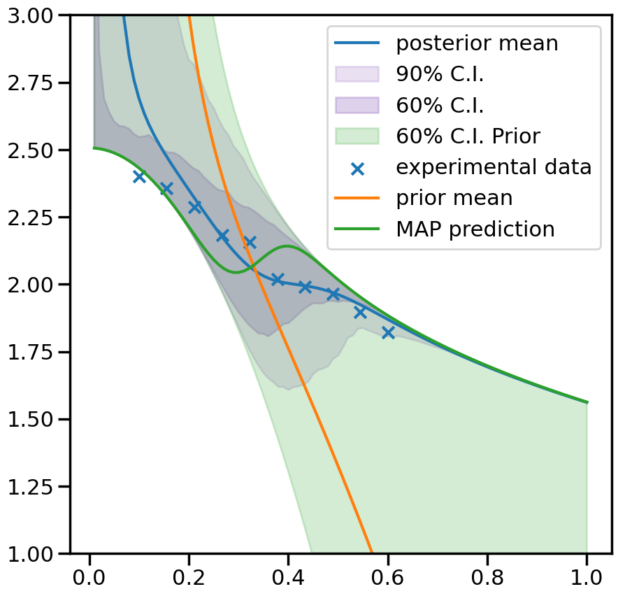
fig, ax = plt.subplots(figsize=(10,10))
ax.plot(plot_g, mean.flatten(), label='posterior mean')
ax.fill_between(plot_g,per5.flatten(),per95.flatten(),color=sns.color_palette()[4], alpha=0.2, label='90% C.I.')
ax.fill_between(plot_g,per20.flatten(),per80.flatten(), color=sns.color_palette()[4], alpha=0.3, label='60% C.I.')
ax.fill_between(plot_g,prior20.flatten(),prior80.flatten(),color=sns.color_palette()[2], alpha=0.2, label='60% C.I. Prior')
ax.scatter(g,exp_data[0], marker='x', label='experimental data')
ax.plot(plot_g, mean_prior.flatten(), label='prior mean')
ax.plot(plot_g, map_prediction.flatten(), label='MAP prediction')
ax.set_ybound(1,3)
ax.legend()

<matplotlib.legend.Legend at 0x7fd188d33210>