1. Ball Drop Example#
This example couples a basic ball drop physics experiment with surmise’s emulators and calibrators to explore a simple yet non-trivial use of surmise. In particular, we will perform calibrations using a data set of experimental height values measured in time with surrogate models of two different parameterized models of the general form \(h(\invar; \psp)\), where \(h\) is the height of the ball above the ground, \(\invar\) represents the independent, or input, variables; \(\psp\), a point in the model’s parameter space.
In the interest of keeping this example concise and clear, the level of care taken to configure, execute, and evaluate the quality of the Bayesian calibration is intentionally overly-simplistic.
Note that we will use scipy.stats to work with different common distributions. Therefore, we adopt that package’s notation and definitions for those distributions.
import numpy as np
import scipy.stats as sps

from surmise.emulation import emulator
from surmise.calibration import calibrator


RNG = np.random.default_rng(39761829560096686505152613678763426794)

EMULATOR_METHOD     = "PCGP"
N_EMU_THETA_SAMPLES = 50
CALIBRATION_METHOD  = "directbayes"
CALIBRATION_ARGS = {
    "sampler":     "metropolis_hastings",
    "theta0":      None,      # Set individually for each model
    "numsamp":     -1,        # Set individually for each model
    "burnSamples": -1,        # Set individually for each model
    "stepType":    "normal",
    "stepParam":   None,      # Set individually for each model
    "verbose":     True
}
1.1. Experimental Setup#
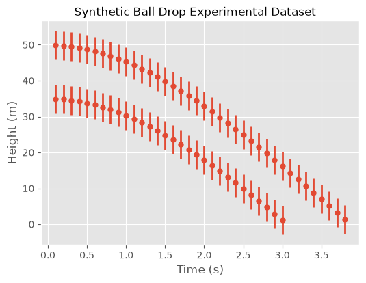
A physicist has an experimental setup that will drop a ball from a given height and subsequently measure the height of the ball above the floor at different times. The experiment is run from two different initial heights to gather the full data set for our calibrations.
H_0_LO = 35.0  # meters
H_0_HI = 50.0  # meters
While this example is contrived, the intent of using two different initial heights is to force the use of the slightly more complex independent variables
which are the initial height of the experiment being measured and the time at which a position measurement is made for that experiment.
X_NAMES = ["h_0_m", "t_s"]
H_0_IDX, T_IDX = (0, 1)
The experimenter believes that the measurement error is the same regardless of the inital height and the height at which measurements were made.
H_VARIANCE = 4.0 # m^2
Rather than perform the actual experiments, we generate synthetic data, which is stored in the DATASET variable, using a model that we believe to be a good representation of the real world and higher-fidelity than the two models that we will use for calibration. This model uses the well-known gravitational constant for objects close to the surface of the Earth and a terminal velocity.
G_STAR          = 9.81   # m/s^2
V_TERMINAL_STAR = 20.0   # m/s
Note that we do not add our own additive measurement noise to the synthetic data despite our assumed non-zero measurement error. Thus, the source of error can be thought of as model specification error, i.e.,, the model is inherently inadequate in representing the synthetic data.
A tabular snippet of the dataset helps visualize the data set’s structure
| height_m | ||
|---|---|---|
| h_0_m | t_s | |
| 35.0 | 0.1 | 34.950970 |
| 0.2 | 34.804114 | |
| 0.3 | 34.560134 | |
| 0.4 | 34.220184 | |
| 0.5 | 33.785849 | |
| ... | ... | ... |
| 50.0 | 3.4 | 8.836529 |
| 3.5 | 6.967717 | |
| 3.6 | 5.087012 | |
| 3.7 | 3.195462 | |
| 3.8 | 1.294028 |
68 rows × 1 columns
and the contents of the single data set are graphed.
1.2. Low-fidelity Model#
Physicists typically assume that acceleration due to gravity near the surface of the Earth, \(g\), is constant. Based on this and assuming that there are no other forces, such as air resistance, acting on the ball, a simple model is
where, contrary to typical notation, \(h_0 > 0\) is an independent variable and \(\psp = g > 0\) is the single unknown parameter for this model.
In particular, this model would be a high-fidelity model if the experiment had been performed in a vacuum such as space. However, we will see that it is indeed a low-fidelity model when fit to data measured in a lab.
def balldropmodel_vacuum(x, theta):
    assert all(theta > 0.0)
    h_0 = x[:, H_0_IDX]
    t   = x[:, T_IDX]
    assert all(h_0 > 0.0)
    assert all(t >= 0.0)

    f = np.zeros((theta.shape[0], len(t)))
    for k in range(f.shape[0]):
        g = theta[k, 0]
        f[k, :] = h_0 - 0.5 * g * (t ** 2)
    return f.T
Since this is a Bayesian calibration, we assume that \(g\) is a random variable and specify a prior distribution for it. To guide the choice of this prior distribution, we know that
\(g > 0\) and
\(g\) is commonly taken to be approximately 10 \(m/s^2\).
A reasonable choice is, therefore,
since its mean is 10 and much of the probability is bunched around this with a slight skew toward smaller accelerations.
class prior_g_vacuum:
    ALPHA = 5.0
    BETA  = 0.5

    def lpdf(theta):
        assert all(theta > 0.0)
        values = sps.gamma.logpdf(theta,
                                  a=prior_g_vacuum.ALPHA,
                                  loc=0.0,
                                  scale=1.0 / prior_g_vacuum.BETA)
        return values.reshape((len(theta), 1))

    def rnd(n):
        samples = sps.gamma.rvs(a=prior_g_vacuum.ALPHA,
                                loc=0.0,
                                scale=1.0 / prior_g_vacuum.BETA,
                                size=n,
                                random_state=RNG)
        return np.reshape(samples, (-1,1))

prior_g_mean, prior_g_var = sps.gamma.stats(
    a=prior_g_vacuum.ALPHA,
    loc=0.0,
    scale=1.0 / prior_g_vacuum.BETA,
    moments="mv"
)
We emulate the low-fidelity model and test the emulator at predetermined times
t_emulator_lo = np.arange(0.0, 3.5, 0.1)
t_emulator_hi = np.arange(0.0, 4.3, 0.1)

x_emulator_vacuum = np.full([len(t_emulator_lo) + len(t_emulator_hi), 2], np.nan, float)
x_emulator_vacuum[:, T_IDX] = np.concatenate(
    (t_emulator_lo, t_emulator_hi)
)
x_emulator_vacuum[:, H_0_IDX] = np.concatenate(
    (H_0_LO * np.ones(len(t_emulator_lo)),
     H_0_HI * np.ones(len(t_emulator_hi)))
)
| h_0_m | t_s | |
|---|---|---|
| 0 | 35.0 | 0.0 |
| 1 | 35.0 | 0.1 |
| 2 | 35.0 | 0.2 |
| 3 | 35.0 | 0.3 |
| 4 | 35.0 | 0.4 |
| ... | ... | ... |
| 73 | 50.0 | 3.8 |
| 74 | 50.0 | 3.9 |
| 75 | 50.0 | 4.0 |
| 76 | 50.0 | 4.1 |
| 77 | 50.0 | 4.2 |
78 rows × 2 columns
and using \(g\) values sampled from our prior.
g_vacuum_train = prior_g_vacuum.rnd(N_EMU_THETA_SAMPLES)

f_vacuum_train = balldropmodel_vacuum(x_emulator_vacuum, g_vacuum_train)

emu_vacuum = emulator(x=x_emulator_vacuum,
                      theta=g_vacuum_train,
                      f=f_vacuum_train,
                      method=EMULATOR_METHOD)

g_vacuum_test = prior_g_vacuum.rnd(N_EMU_THETA_SAMPLES)
f_vacuum_test = balldropmodel_vacuum(x_emulator_vacuum, g_vacuum_test)

pred_vacuum = emu_vacuum.predict(x=x_emulator_vacuum, theta=g_vacuum_test)
pred_vacumm_m, pred_vacuum_var = pred_vacuum.mean(), pred_vacuum.var()

display(Math(r'R^2 = {:.3f}'.format(1 - np.sum(np.square(pred_vacumm_m - f_vacuum_test))/np.sum(np.square(f_vacuum_test.T - np.mean(f_vacuum_test, axis = 1))))))
print('Root Mean Squared Error = {:.3f}'.format(np.sqrt(np.mean(np.square(pred_vacumm_m - f_vacuum_test)))))
Root Mean Squared Error = 0.184
g_0 = prior_g_mean

print()
print("Prior distribution characterization")
print("-" * 80)
print(f"Mean g = {prior_g_mean} m/s^2")
print(f"Std  g = {np.sqrt(prior_g_var)} m/s^2")
print()
print("Calibration starting point")
print("-" * 80)
print(f"g = {g_0} m/s^2")
print()

args = CALIBRATION_ARGS.copy()
args["theta0"]      = np.array([[g_0]])
args["numsamp"]     = 1000
args["burnSamples"] = 1000
args["stepParam"]   = np.array([0.2])

cal_vacuum = calibrator(
    emu=emu_vacuum,
    x=DATASET["x"], y=DATASET["y"], yvar=DATASET["yvar"],
    thetaprior=prior_g_vacuum,
    method=CALIBRATION_METHOD, args=args
)
Prior distribution characterization
--------------------------------------------------------------------------------
Mean g = 10.0 m/s^2
Std  g = 4.47213595499958 m/s^2

Calibration starting point
--------------------------------------------------------------------------------
g = 10.0 m/s^2
Final Acceptance Rate: 0.446
We have access to the estimate of the posterior distribution and can use it to access summary statistics
posterior_mean = cal_vacuum.theta.mean()
posterior_std = np.sqrt(cal_vacuum.theta.var())

print()
print(f"g posterior mean = {posterior_mean[0]}")
print(f"g posterior std  = {posterior_std[0]}")
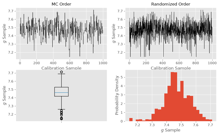
g posterior mean = 7.468910265257051
g posterior std  = 0.09084062413195643
Therefore, the Bayesian analysis resulted in a posterior that is much narrower than the prior and shifted both from the mean and mode of the prior as well from the true value of \(g\), which might be expected since we have used the low-fidelity model.
We can also access the samples used by the calibration process
in the order in which they were sampled and
with a randomized ordering
for visualizing some aspects of the calibration process.
samples_MC_vacuum         = cal_vacuum.info["thetarnd"]
samples_randomized_vacuum = cal_vacuum.theta.rnd(args["numsamp"])
cal_vacuum_post = cal_vacuum.predict(DATASET["x"])
rndm_vacuum_m = cal_vacuum_post.rnd(s = 1000)

fig = plt.figure(4, figsize=(4, 3))

subp = fig.add_subplot(111)
subp.set_title("Low-fidelity Model", fontsize=FONTSIZE)
for k in (H_0_LO, H_0_HI):
    inds = np.where(DATASET["x"][:, H_0_IDX] == k)[0]
    upper = np.percentile(rndm_vacuum_m[:, inds], 97.5, axis=0)
    lower = np.percentile(rndm_vacuum_m[:, inds],  2.5, axis=0)
    subp.fill_between(DATASET["x"][inds, T_IDX], lower, upper, color = 'blue', alpha=0.25)
    subp.plot(DATASET["x"][inds, T_IDX], DATASET["y"][inds], 'k.', markersize = 5)
subp.set_xlabel("Time (s)", fontsize=FONTSIZE)
subp.set_ylabel("Height (m)", fontsize=FONTSIZE)
subp.tick_params(axis="both", labelsize=TICK_FONTSIZE)
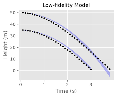
While the fit to the low initial ball height expertimental data is not so bad, the disagreement between model and data degrades for large times for the higher initial ball height data. This further suggests that the low-fidelity model is poor.
1.3. High-fidelity Model#
To better represent the physics of this laboratory experiment, the physicist specifies a second model that attempts to account for the effect of air resistance on the ball by assuming that after some time \(t_{ter} > 0\) the ball will move linearly with terminal speed \(v_{ter} > 0\) due to the balancing of the forces of air resistance and gravity on the ball or
where
\(h_0 > 0\) is still the initial height of the ball above the ground at time \(t=0\) and
\(c_{ter} > 0\) is the distance traveled by the ball in time \(t_{ter}\).
The unknown parameters for this problem are \(\psp = (c_{ter}, v_{ter})\).
C_TER_IDX, V_TER_IDX = (0, 1)
THETA_NAMES = ["$c_{ter}$", r"$v_{ter}$"]
While an improvement, this model is still flawed. For example, the model should only be used for \(t \ge t_{ter}\).
T_TERMINAL = 2.0  # seconds

def balldropmodel_air(x, theta):
    h_0 = x[:, H_0_IDX]
    t   = x[:, T_IDX]
    assert all(h_0 > 0.0)
    assert all(t >= T_TERMINAL)
    assert all(theta.flatten() > 0.0)
    c_ter = theta[:, C_TER_IDX]
    v_ter = theta[:, V_TER_IDX]

    f = np.zeros((theta.shape[0], x.shape[0]))
    for k in range(f.shape[0]):
        f[k, :] = h_0 - c_ter[k] - v_ter[k] * (t - T_TERMINAL)
    return f.T
Since this is a Bayesian treatment, we assume that \(c_{ter}, v_{ter}\) are random variables and specify a joint prior distribution for them. If the relationship among the unknown parameters is known, one may suggest a prior distribution that encodes correlation. Otherwise, an independence assumption may be assumed, as done below.
To determine this, we know that \(v_{ter}\) must be positive. Since the low-fidelity model has only gravity acting on the ball and the high-fidelity model has the additional force of air resistance countering gravity, we hope that the low-fidelity model predicts a larger displacement than the high-fidelity model at each time. Therefore, we suspect that
We assume that the two random variables are independent and specify the (hopefully) reasonable marginal prior distributions
\(v_{ter} \sim \Gamma(\alpha=5, \beta=1/3)\) and
\(c_{ter} \sim \mathcal{U}_{[0, h_0 - h_{vac}(h_0, t_{ter}; \E[g])]}\).
x_ter = np.full([1, 2], np.nan, float)
x_ter[0, H_0_IDX] = H_0_HI
x_ter[0, T_IDX] = T_TERMINAL

theta = np.array([[prior_g_mean]])

max_displacement_t_ter = H_0_HI - balldropmodel_vacuum(x_ter, theta)[0][0]

class prior_theta_air:
    C_LO = 0.0
    C_HI = max_displacement_t_ter

    V_ALPHA = 5.0
    V_BETA  = 1.0 / 3.0

    def lpdf(theta):
        assert all(theta.flatten() > 0.0)
        c_values = sps.uniform.logpdf(theta[:, C_TER_IDX],
                                      loc=prior_theta_air.C_LO,
                                      scale=prior_theta_air.C_HI - prior_theta_air.C_LO)
        v_values = sps.gamma.logpdf(theta[:, V_TER_IDX],
                                    a=prior_theta_air.V_ALPHA,
                                    loc=0.0,
                                    scale=1.0 / prior_theta_air.V_BETA)
        return (c_values + v_values).reshape((len(theta), 1))

    def rnd(n):
        samples = np.full([n, 2], np.nan, float)
        samples[:, C_TER_IDX] = sps.uniform.rvs(
            loc=prior_theta_air.C_LO,
            scale=prior_theta_air.C_HI - prior_theta_air.C_LO,
            size=n,
            random_state=RNG
        )
        samples[:, V_TER_IDX] = sps.gamma.rvs(
            a=prior_theta_air.V_ALPHA,
            loc=0.0,
            scale=1.0 / prior_theta_air.V_BETA,
            size=n,
            random_state=RNG
        )
        return samples

prior_c_ter_mean = 0.5 * (prior_theta_air.C_LO + prior_theta_air.C_HI)
prior_c_ter_var  = (prior_theta_air.C_HI - prior_theta_air.C_LO)**2 / 12.0

prior_v_ter_mean = prior_theta_air.V_ALPHA / prior_theta_air.V_BETA
prior_v_ter_var  = prior_theta_air.V_ALPHA / prior_theta_air.V_BETA**2
We emulate the high-fidelity model and test the emulator at predetermined times
t_emulator_lo = np.arange(T_TERMINAL, 3.5, 0.1)
t_emulator_hi = np.arange(T_TERMINAL, 4.3, 0.1)

x_emulator_air = np.full([len(t_emulator_lo) + len(t_emulator_hi), 2], np.nan, float)
x_emulator_air[:, T_IDX] = np.concatenate(
    (t_emulator_lo, t_emulator_hi)
)
x_emulator_air[:, H_0_IDX] = np.concatenate(
    (H_0_LO * np.ones(len(t_emulator_lo)),
     H_0_HI * np.ones(len(t_emulator_hi)))
)
| h_0_m | t_s | |
|---|---|---|
| 0 | 35.0 | 2.0 |
| 1 | 35.0 | 2.1 |
| 2 | 35.0 | 2.2 |
| 3 | 35.0 | 2.3 |
| 4 | 35.0 | 2.4 |
| ... | ... | ... |
| 33 | 50.0 | 3.8 |
| 34 | 50.0 | 3.9 |
| 35 | 50.0 | 4.0 |
| 36 | 50.0 | 4.1 |
| 37 | 50.0 | 4.2 |
38 rows × 2 columns
and using \(c_{ter}, v_{ter}\) values sampled from our prior.
theta_air_train = prior_theta_air.rnd(N_EMU_THETA_SAMPLES)

f_air_train = balldropmodel_air(x_emulator_air, theta_air_train)

emu_air = emulator(x=x_emulator_air,
                   theta=theta_air_train,
                   f=f_air_train,
                   method=EMULATOR_METHOD)

theta_air_test = prior_theta_air.rnd(N_EMU_THETA_SAMPLES)
f_air_test = balldropmodel_air(x_emulator_air, theta_air_test)

pred_air = emu_air.predict(x=x_emulator_air, theta=theta_air_test)
pred_air_m, pred_air_var = pred_air.mean(), pred_air.var()

display(Math(r'R^2 = {:.3f}'.format(1 - np.sum(np.square(pred_air_m - f_air_test))/np.sum(np.square(f_air_test.T - np.mean(f_air_test, axis = 1))))))
print('Root Mean Squared Error = {:.3f}'.format(np.sqrt(np.mean(np.square(pred_air_m - f_air_test)))))
Root Mean Squared Error = 0.008
Since this model is valid only once the ball has acheived terminal velocity, we will only calibrate the model using data acquired with \(t \ge t_{ter}\). After the calibration is done, we should check if the calibration results are at least consistent with the modeler’s choice of \(t_{ter}\).
indices = np.where(DATASET["x"][:, T_IDX] >= T_TERMINAL)

theta_0 = np.full(2, np.nan, float)
step_size = theta_0.copy()

theta_0[C_TER_IDX] = prior_c_ter_mean
theta_0[V_TER_IDX] = prior_v_ter_mean

step_size[C_TER_IDX] = 0.25
step_size[V_TER_IDX] = 1.0

print()
print("Marginal prior distribution characterizations")
print("-" * 80)
print(f"Mean c_ter = {prior_c_ter_mean} m")
print(f"Std  c_ter = {np.sqrt(prior_c_ter_var)} m")
print()
print(f"Mean v_ter = {prior_v_ter_mean} m/s")
print(f"Std  v_ter = {np.sqrt(prior_v_ter_var)} m/s")
print()
print("Calibration starting point")
print("-" * 80)
print(f"c_ter = {theta_0[C_TER_IDX]} m")
print(f"v_ter = {theta_0[V_TER_IDX]} m/s")
print()

args = CALIBRATION_ARGS.copy()
args["theta0"]      = theta_0.reshape(1, len(theta_0))
args["numsamp"]     = 10000
args["burnSamples"] = 1000
args["stepParam"]   = step_size

cal_air = calibrator(
    emu=emu_air,
    x=DATASET["x"][indices],
    y=DATASET["y"][indices],
    yvar=DATASET["yvar"][indices],
    thetaprior=prior_theta_air,
    method=CALIBRATION_METHOD, args=args
)

# Access data for studying calibration as for low-fidelity model
posterior_mean_air = cal_air.theta.mean()
c_ter_posterior_mean = posterior_mean_air[C_TER_IDX]
v_ter_posterior_mean = posterior_mean_air[V_TER_IDX]
posterior_std_air = np.sqrt(cal_air.theta.var())
c_ter_posterior_std = posterior_std_air[C_TER_IDX]
v_ter_posterior_std = posterior_std_air[V_TER_IDX]

samples_MC_air         = cal_air.info["thetarnd"]
samples_randomized_air = cal_air.theta.rnd(args["numsamp"])
Marginal prior distribution characterizations
--------------------------------------------------------------------------------
Mean c_ter = 10.0 m
Std  c_ter = 5.773502691896258 m

Mean v_ter = 15.0 m/s
Std  v_ter = 6.708203932499369 m/s

Calibration starting point
--------------------------------------------------------------------------------
c_ter = 10.0 m
v_ter = 15.0 m/s
Final Acceptance Rate: 0.3971
c_ter posterior mean = 16.551416860615486
c_ter posterior std  = 0.6880236880355045

v_ter posterior mean = 17.513678635241135
v_ter posterior std  = 0.7356000335401081
The calibration has resulted in marginal posterior distributions that are narrower than for the marginal priors and that have each shifted a bit from the means of the marginal priors.
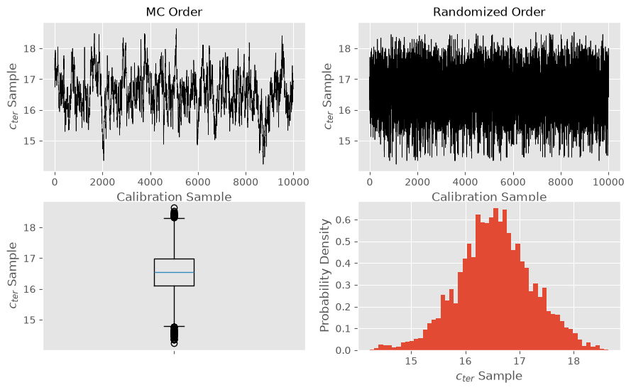
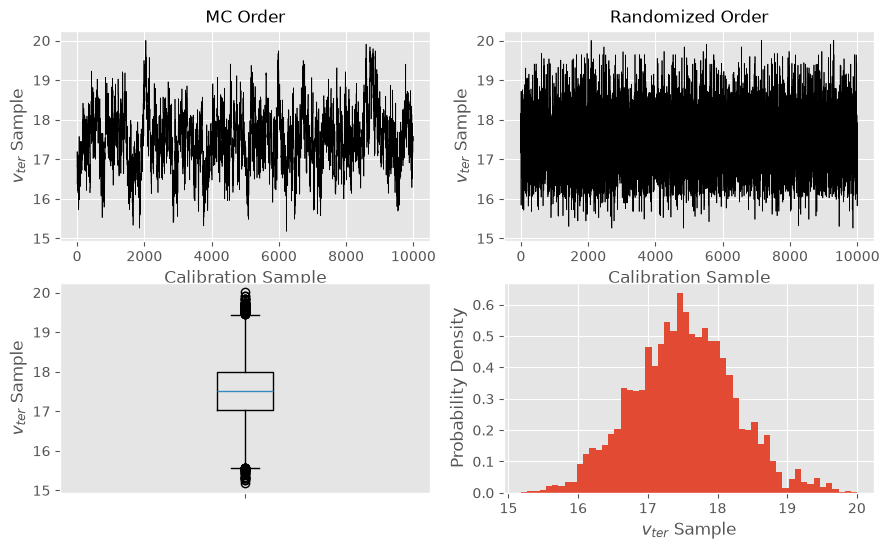
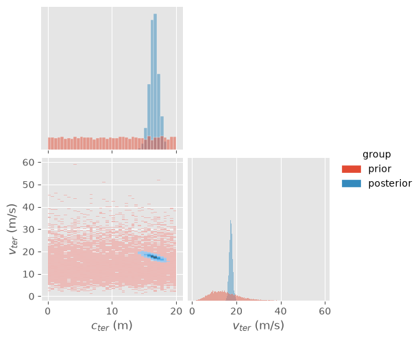
Happily, the supports of the marginal posterior distributions are consistent with the lower and upper limits discussed when defining the prior distribution. Note that the true value for the terminal velocity is in the upper tail of the marginal posterior distribution. While this could be due to a insufficiency in our calibration procedure, it could also indicate that the high-fidelity model is still a poor model for physical reality.
The MC ordered sample plots indicate an anticorrelation between the two parameters, which is seen more clearly in the histogram of the joint posterior distribution in the corner plot.
indices = np.where(DATASET["x"][:, T_IDX] >= T_TERMINAL)
dataset_x_ter = DATASET["x"][indices]

cal_air_post = cal_air.predict(dataset_x_ter)
rndm_air_m = cal_air_post.rnd(s = 1000)

fig = plt.figure(9, figsize=(4, 3))

subp = fig.add_subplot(111)
subp.set_title("With air-resistance", fontsize=FONTSIZE)

for k in (H_0_LO, H_0_HI):
    inds = np.where(np.squeeze(dataset_x_ter[:, H_0_IDX] == k))[0]
    upper = np.percentile(rndm_air_m[:, inds], 97.5, axis = 0)
    lower = np.percentile(rndm_air_m[:, inds], 2.5, axis = 0)
    subp.fill_between(dataset_x_ter[inds, T_IDX], lower, upper, color = 'blue', alpha=0.25)
    subp.plot(DATASET["x"][:, T_IDX], DATASET["y"], 'k.', markersize = 5)

subp.axvline(T_TERMINAL, color="black", linestyle=":", label=r"$t_{ter}$")
subp.set_xlabel("Time (s)", fontsize=FONTSIZE)
subp.set_ylabel("Height (m)", fontsize=FONTSIZE)
subp.tick_params(axis="both", labelsize=TICK_FONTSIZE)
_ = subp.legend(loc="best", fontsize=FONTSIZE)
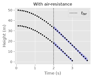
For this higher-fidelity calibration, the posterior predictions for \(t \ge t_{ter}\) are much better than the low-fidelity model predictions as expected.